ASReml-R Quick Reference

Data for analysis using ASReml-R are generally contained in a text file or a spreadsheet and are read into a data frame using the appropriate R functions.

Character fields and numeric fields are often not treated as factors, and you must manually convert them into factors as required.

The function asreml.read.table() reads data from a text file and automatically converts variates whose names begin with a capital letter in the header line into factors.

ASReml-R uses the Wilkinson and Rogers (1973) notation. The model term A:B denotes an interaction or nested effect depending on which other terms are previously included in the model.

An example of the asreml() call for a simple randomized complete block (RCB) design using nin89 dataframe.

The fixed terms (required) is specified as a formula with the numerical response (yield) on the left of a ∼ operator and the fixed factor (Variety) on the right.

In random and residual the factors (Rep and units) are positioned after the ∼ operator; units is an internal experimental unit factor; and idv() is the homogeneous identity variance structure.

Missing values are allowed in design factors when x = "include". And response records with missing values in the response are included by default with y = "include".

The formula here specifies: response, fixed factors, interactions and covariates.

If the response term specified is several columns, then a multivariate/multitrait analysis is performed.

Each random term needs to be associated to a variance model, idv() is used by default. The examples below use autoregressive matrices for both rows and columns.

In the previous example, the spatial model is defined as a G structure, and in the following example, it is defined as an R structure.

The conditional factor at() is used when another factor depends on specific levels on this factor.

dsum() is available only for the residual formula and specifies a direct sum, one for each level of the conditioning factor.

ASReml-R has a wide range of variance models that can be used to specify the variance matrix of terms in the random and residual formulae. Some of them are shown below:

The class of general variance models also includes cor, corb, corg, chol, cholc, ante and the factor analytic structure (fa, sfa, facv, rr).

The function ainverse() uses the method of Meuwissen and Luo (1992) to compute the inverse of the numerator relationship matrix (NRM) directly from pedigree.

With no arguments, asreml.options() returns a list of settings that can be altered. The full list can be displayed by typing help(asreml.options)

The settings are maintained per R session.

Weighted analyses are achieved by using the weights argument within function asreml()

The inclusion of argument family allows for specifying other probability distributions, fitting what is referred to as a Generalized Linear Mixed Model (GLMM).

The options are Gaussian, Gamma, Poisson, Binomial and Negative Binomial.

The update() function can be used if the model requires further interactions or modifications.

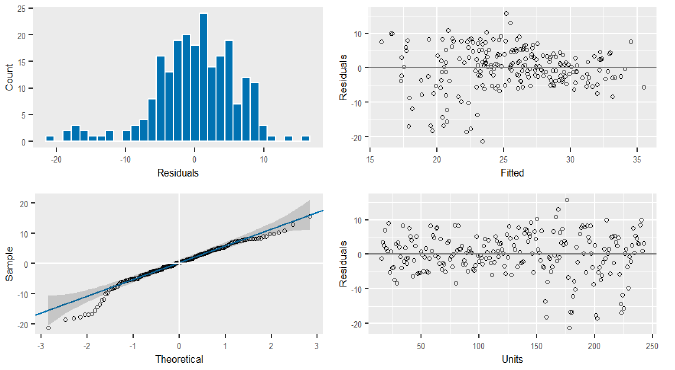
The plot() function used with an asreml object will produce the following four residual plots:

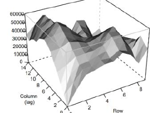
For spatial models the varioGram() will also produce a diagnostic plot.

The summary() function returns a list with a range of components, such as:

The coefficients from the fixed and random parts of the model are available in the coef.fixed and coef.random or using coef().

The basic tool for fixed effects inference is the wald(), and ANOVA-like table. The asymptotic version is obtained as:

The version that obtains degrees of freedom is:

Function used to compare nested models based on the REML likelihood ratio test implemented with the function lrt()

The predict() method obtains an estimated or predicted values (means) for an element of interest.

The average standard error of difference (SED) between the predicted means is:

The option vpredict() allows to define functions of variance components and their SEs. These are represented by the strings "V1","V2",. . .