ASReml-Python 1.0.0 · Updated 2026-10

ASReml-Python Quick Reference

Everything you need at your fingertips — from reading data and writing model formulae to variance structures, tests and predictions. Copy any snippet straight into Python.

Printable 2-page PDF

Download PDF

Fitting a model

Importing ASReml, reading data, model formulae and a first fit.

Importing ASReml

import asreml

from asreml import (asreml, ainverse,

define_categorical_variables, residual_plot,

variogram)

Reading Data

Data for analysis using ASReml-Python are generally contained in a text file or a spreadsheet and are read into a data frame using the Pandas package.

import pandas as pd

nin89 = pd.read_csv("/path/nin89.csv",

sep = ",", header = 0)

	Variety	Id	pid	raw	Rep	nloc	yield	lat	long	Row	Column
16	LANCER	1	1101	585	1	4	29.25	4.3	19.2	16	1
17	BRULE	2	1102	631	1	4	31.55	4.3	20.4	17	1
18	REDLAND	3	1103	701	1	4	35.05	4.3	21.6	18	1
19	CODY	4	1104	602	1	4	30.1	4.3	22.8	19	1
20	ARAPAHOE	5	1105	661	1	4	33.05	4.3	24	20	1
21	NE83404	6	1106	605	1	4	30.25	4.3	25.2	21	1

Character fields and numeric fields are often not treated as factors, and you must manually convert them into factors.

nin89 = define_categorical_variables(nin89,

variables = ["Variety", "Rep", "Row", "Column"])

Model formulae

ASReml-Python uses the Wilkinson and Rogers (1973) notation. The model term A:B denotes an interaction or nested effect depending on which other terms are previously included in the model.

asreml(

response = "y",

fixed = "Site",

random = "Genotype + Site:Genotype",Use + to add model terms · “:” denotes interaction

data = my_data)

asreml(

response = "y",

fixed = "Site",

random = "Site:Genotype",“:” denotes nested effect

data = my_data)

A first model (RCB design)

An example of the asreml() call for a simple randomized complete block (RCB) design using the nin89 dataframe is shown below.

nin89_asr = asreml(

response = "yield",

fixed = "Variety",

random = "idv(Rep, init = 10)",Set initial values (optional)

residual = "units",

options = {"na_action":

{"x": "include", "y": "include"}},

predict = {"classify": "Variety"},

vpredict = {"ICC": "V2/(V1+V2)"},

data = nin89)

The response, fixed, random and residual terms are specified as string (use quotation marks) based on the column names in the dataset.

In residual, units is an internal experimental unit factor; and idv() is the homogeneous identity variance structure (see Variance Models).

The options receives a dictionary with internal arguments; e.g. "na_action", where: "x": "include" allows missing values in the design factors and "y": "include" response records with missing values are included.

Model terms

Response, fixed, random and residual terms.

Response Terms

The formula can specify univariate or multivariate models.

asreml(response = "y", ...)univariate form

asreml(multivariate general mean

response = ["y1",..., "yk"],

fixed = "trait + x + trait:x", ...)“trait” is a reserved word

Fixed Terms

The formula can specify fixed factors, interactions and covariates.

asreml(..., fixed = "Variety", ...)intercept plus Variety

asreml(..., fixed = "-1 + Variety", ...)-1 removes the intercept

asreml(..., fixed = "1", ...)intercept-only

Random and Residual terms

Each random term needs to be associated to a variance model, idv() is assumed by default. The examples below use autoregressive matrices for both rows and columns.

asreml(...,

random = "ar1v(Column):ar1(Row)",ar1v() is a variance model · ar1() is a correlation model

residual = "idv(units)",

....)

In the previous example, the spatial model is defined as part of the G structure, and in the following example, it is defined as part of the R structure.

nin89_spt = asreml(

response = "yield",

fixed = "Variety",

random = "idv(Rep)",

residual = "ar1v(Column):ar1(Row)",The operator “:” applies the direct product structure

options = {"na_action":

{"x": "include","y": "include"}},

data = nin89)

Initial values & conditional factors

Editing starting values and conditioning terms on factor levels.

Initial Values

The fit_options and .initial_values return a dictionary holding of the variance components.

asreml(...,

fit_options = {"process_stage":"preprocess"} )

init = nin89_asr.initial_values(display = True)

The values can be modified:

init["idv(Rep)!IDV_V"]["value"] = 0.5

The .fit method runs the model with new values.

nin89_asr.fit(initial_values = init)

Conditional Factors

The conditional factor at() is used when another factor depends on specific levels on this factor.

asreml(...,

random = "at(Site, 1):Block",

residual = "dsum( units, Site)" , ....)

dsum() is available only for the residual formula and specifies a direct sum, one for each level of the conditioning factor.

Variance models

Structures for the random and residual formulae.

Common variance models

ASReml-Python has a wide range of variance models that can be used to specify the variance matrix of terms in the random and residual formulae. Some of them are shown below:

σ²

1000010000100001

idv

identity

σ₁²0000σ₂²0000σ₃²0000σ₄²

idh or diag

diagonal

σ²

1ρρρρ1ρρρρ1ρρρρ1

corv

uniform homogeneous

corh

uniform heterogeneous

ar1

1st order autocorrelation

corgh or us

unstructured

The class of general variance models also includes cor, corb, corg, chol, cholc, ante and factor analytic structures (fa, sfa, facv, rr).

Relationships, GLMM & weights

Pedigree matrices, other distributions and weighted analyses.

Adding a Relationship Matrix

The function ainverse() computes the inverse of the numerator relationship matrix from provided pedigree.

harvey_ped = pd.read_csv("./harvey_ped.csv")

harvey_ai = ainverse(harvey_ped)

	Calf	Sire	Dam
0	Sire_1	0	0
1	Sire_2	0	0
2	Sire_3	0	0
3	Sire_4	0	0
4	Sire_5	0	0

	rowid	colid	vals
0	1	1	3.666667
1	2	2	3.666667
2	3	3	2.666667
3	4	4	3.666667
4	5	5	3.333333

The variance model function vm() allows the use of the inverse of a numerator relationship matrix or one generated from a genomics data.

adg_asr = asreml(

response = "y3",

fixed = "Line",

random = "vm(Calf, harvey_ai)",vm = variance model function · Calf = reference factor · harvey_ai = Ainv matrix

residual = "units",

data = {"data": harvey, "harvey_ai": harvey_ai})

GLMM

The inclusion of argument family allows for specifying other probability distributions, fitting what is referred to as a Generalized Linear Mixed Model (GLMM).

binnor_asr = asreml(

response = "surv",

fixed = "Sex + Grp",

random = "Sire",

family = "binomial(link = logit, dispersion = 1)",

data=binnor)

The family options are: gaussian, gamma, poisson, binomial and negative_binomial.

Weights

Weighted analyses are implemented by using the weights argument within function asreml().

asreml(..., weights = "wt", ...)variate in the data frame

Plotting

Residual diagnostics and the spatial variogram.

Residual Plots

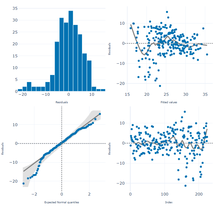
The residual_plot() function used with an asreml object will produce the following four residual plots:

residual_plot(nin89_asr)

Four residual diagnostic plots: histogram of residuals, residuals vs fitted values, normal Q-Q plot and residuals vs index

Variogram

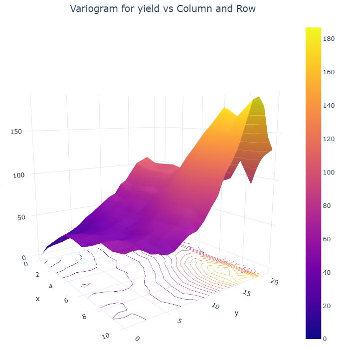
For spatial models the variogram() will also produce a diagnostic plot based on the spatial model fitted.

variogram(nin89_spt)

3D variogram surface for yield vs Column and Row

Extracting output

Summary statistics, variance components and solutions.

Summary

The summary() function returns a list with a variety of elements, such as:

nin89_asr.summary()["loglik"]log-likelihood value

-454.4691

nin89_asr.summary()["varcomp"]variance components table

	gamma	sigma	std.error	bounds	%ch
idv(units)!units!SCA_V	1.000000	49.582380	5.458841	P	0
idv(Rep)!Rep!ID_V	0.199323	9.882913	8.792661	P	0

nin89_asr.summary()["aic"]Akaike Information Criterion

912.9382

nin89_asr.summary()["bic"]Bayesian Information Criterion

919.1861

Solutions

The coefficients (or solutions) from solving the mixed model equations for the fixed and random parts of the model are in .coefficients().

nin89_asr.coefficients()

	estimate	standard_error
Variety_ARAPAHOE	0.0000	0.000000
Variety_BRULE	-3.3625	4.979075
Variety_BUCKSKIN	-3.8750	4.979075
Variety_CENTURA	-7.7875	4.979075
Variety_CENTURK78	0.8625	4.979075

Inference & prediction

Wald tests, predicted means and functions of variances.

Wald Test

The basic tool for fixed effects inference is the Wald (ANOVA-like) table. The option that calculates degrees of freedom is:

asreml(..., options = {"wald":

{"den_df": "numeric",

"ss_type": "conditional"}}, ...)

nin89_asr.wald()

	NumDF	DenDF	F-inc	F-con	M	P-con
mu	1	3.0	242.057101	242.057101	.	0.000577
Variety	55	165.0	0.875490	0.875490	A	0.711853

Predict

The predict method obtains estimated or predicted means for an element or factor of interest.

asreml(...,

predict = {"classify": "Variety"} , ...)

nin89_asr.predict()

	Variety	Pred Values	s.e.	Ecode
0	ARAPAHOE	29.4375	3.855683	E
1	BRULE	26.0750	3.855683	E
2	BUCKSKIN	25.5625	3.855683	E
3	CENTURA	21.6500	3.855683	E

Functions of Variances

The vpredict allows to define functions of variance components and estimate their standard error. These are represented by the strings "V1", "V2"…

asreml(...,

vpredict = {"ICC": "V2/(V1+V2)"} , ...)

nin89_asr.vpredict()Intra-block correlation

	estimate	std.error
ICC	0.166196	0.124396

Keep it on your desk

Download the printable two-page ASReml-Python Quick Reference.

Download PDF